MATLAB-ROS Interface

Note

The Interbotix MATLAB-ROS Interface requires that the ROS Interface has already been installed.

For usage and structure information on the MATLAB interface that builds on top of ROS, check out the MATLAB Demos page. Further documentation of the MATLAB API’s functionality can be found on this page. Note that you can check the source code methods’ docstrings for information on each method.

Note

Using this interface requires that your machine has Python 2.7 if your ROS distribution is Melodic or Python 3.9 if your ROS distribution is Noetic. You may be able to run if your Python’s major version matches what’s required. Visit MATLAB’s ROS System Requirements page for more information.

Attention

The MATLAB-ROS API is not compatible with Gazebo-simulation robots.

Attention

The MATLAB-ROS API is currently only compatible with the ROS 1 interface. ROS 2 support is not planned at this time.

Setup

Before you are able to use the MATLAB-ROS API, you must first build the Interbotix messages and setup your MATLAB workspace. Convenience scripts have been provided to make this process easier.

Building the Interbotix ROS Messages

Note

You only have to build the Interbotix ROS messages once in a workspace.

The process for building the messages is as follows:

1. Open MATLAB.
2. Navigate to the matlab_demos directory.
3. Run the function interbotix_build_ros1_messages from your MATLAB console. Make sure that you have not run the pyenv command before doing so.
4. The script will perform the following actions to build the messages and test that they work properly:
   1. Check that Interbotix custom messages do not already exist on your machine.
   2. Run rosgenmsg() in the interbotix_ros_core/interbotix_ros_xseries directory. This process might take a few minutes. The process of building ROS messages in MATLAB is documented on MathWorks’ website in the articles Create Custom Messages from ROS Package and ROS Custom Message Support.
   3. Add the directory in which the messages were build to the MATLAB path and save it.
   4. Clear all classes and rehash the toolbox cache.
   5. Check that an interbotix_xs_msgs/ message appears in the list generated from the rosmsg("list") command.
   6. If this process works, the function will return true. Otherwise, it will return false with a message.
5. Close MATLAB.

Setting up your MATLAB Workspace

Note

You must follow this process every time you open a new session of MATLAB. See Making Startup Easier for tips on simplifying this process.

The process for setting up your MATLAB workspace is as follows:

1. Open MATLAB.
2. Navigate to the matlab_demos directory.
3. Run the function interbotix_matlab_ros_setup() from your MATLAB console.
4. The script will perform the following actions to setup your workspace and test that the demos will work.
   1. Add the Interbotix ROS messages to the MATLAB path.
   2. Add the Interbotix xs modules to the MATLAB path.
   3. Add the Modern Robotics MATLAB library to the MATLAB path.
   4. If this process works, the function will return true. Otherwise, it will return false with a message.
5. You can now run the demo MATLAB scripts, or develop your own.

Terminology

Transforms

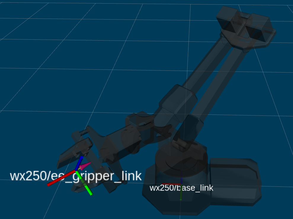
End-effector poses are specified from /<robot_name>/ee_gripper_link (a.k.a the ‘Body’ frame) to /<robot_name>/base_link (a.k.a the ‘Space’ frame). In the code documentation, this transform is knows as T_sb (i.e. the transform that specifies the ‘Body’ frame ‘b’ in terms of the ‘Space’ frame ‘s’). In the image above, you can see both of these frames. The X axes are in red, the Y axes are in green, and the Z axes are in blue. The rotation and translation information is stored in a homogeneous transformation matrix.

\[\begin{split}T = \begin{bmatrix} R & p \\ 0 & 1 \end{bmatrix} = \begin{bmatrix} r_{11} & r_{12} & r_{13} & p_1 \\ r_{21} & r_{22} & r_{23} & p_2 \\ r_{31} & r_{32} & r_{33} & p_3 \\ 0 & 0 & 0 & 1 \\ \end{bmatrix}\end{split}\]

In a homogeneous transformation matrix, the first three rows and three columns \(R\) define a 3-dimensional rotation matrix that describes the orientation of the ‘Body’ frame with respect to the ‘Space’ frame. The first three rows and the fourth column \(p\) of the matrix represent the translational position (i.e. xyz) of the ‘Body’ frame with respect to the ‘Space’ frame. The fourth row of the matrix is always [0 0 0 1] for matrix multiplication purposes.

You will see two other homogeneous transformation matrices in the code: T_sd and T_sy. T_sd defines the desired end-effector pose with respect to the ‘Space’ frame. This transformation is used in methods like set_ee_pose_matrix, where a single desired pose is to be solved for. T_sy is a transform from the ‘Body’ frame to a virtual frame with the exact same x, y, z, roll, and pitch as the ‘Space’ frame. However, it contains the ‘yaw’ of the ‘Body’ frame. Thus, if the end-effector is located at xyz = [0.2, 0.2, 0.2] with respect to the ‘Space’ frame, this converts to xyz = [0.2828, 0, 0.2] with respect to the virtual frame of the T_sy transformation. This convention helps simplify how you think about the relative movement of the end-effector. The method set_ee_cartesian_trajectory uses T_sy to command relative movement of the end-effector using the end-effector’s yaw as a basis for its frame of reference.

Timing Parameters

The MATLAB API uses four different timing parameters to shape the time profile of movements.

The first two parameters are used to determine the time profile of the arm when completing moves from one pose to another. These can be set in the constructor of the object, or by using the set_trajectory_time method.

• moving_time - duration in seconds it should take for all joints in the arm to complete one move.
• accel_time - duration in seconds it should take for all joints in the arm to accelerate/decelerate to/from max speed.

The second two parameters are used to define the time profile of waypoints within a trajectory. These are used in functions that build trajectories consisting of a series of waypoints such as set_ee_cartesian_trajectory.

• wp_moving_time - duration in seconds that each waypoint in the trajectory should move.
• wp_accel_time - duration in seconds that each waypoint in the trajectory should be accelerating/decelerating (must be equal to or less than half of wp_moving_time).

Functions

set_ee_pose_matrix

set_ee_pose_matrix allows the user to specify a desired pose in the form of the homogeneous transformation matrix, T_sd. This method attempts to solve the inverse kinematics of the arm for the desired pose. If a solution is not found, the method returns False. If the IK problem is solved successfully, each joint’s limits are checked against the IK solver’s output. If the solution is valid, the list of joint positions is returned. Otherwise, False is returned.

Warning

If an IK solution is found, the method will always return it even if it exceeds joint limits and returns False. Make sure to take this behavior into account when writing your own scripts.

set_ee_pose_components

Some users prefer not to think in terms of transformation or rotation matrices. That’s where the set_ee_pose_components method comes in handy. In this method, you define T_sd in terms of the components it represents - specifically the x, y, z, roll, pitch, and yaw of the ‘Body’ frame with respect to the ‘Space’ frame (where x, y, and z are in meters, and roll, pitch and yaw are in radians).

Note

If using an arm with less than 6dof, the ‘yaw’ parameter, even if specified, will always be ignored.

set_ee_cartesian_trajectory

When specifying a desired pose using the methods mentioned above, your arm will its end-effector to the desired pose in a curved path. This makes it difficult to perform movements that are ‘orientation-sensitive’ (like carrying a small cup of water without spilling). To get around this, the set_ee_cartesian_trajectory method is provided. This method defines a trajectory using a series of waypoints that the end-effector should follow as it travels from its current pose to the desired pose such that it moves in a straight line. The number of waypoints generated depends on the duration of the trajectory (a.k.a moving_time), along with the period of time between waypoints (a.k.a wp_period). For example, if the whole trajectory should take 2 seconds and the waypoint period is 0.05 seconds, there will be a total of 2/0.05 = 40 waypoints. Besides for these method arguments, there is also wp_moving_time and wp_accel_time. Respectively, these parameters refer to the duration of time it should take for the arm joints to go from one waypoint to the next, and the time it should spend accelerating while doing so. Together, they help to perform smoothing on the trajectory. If the values are too small, the joints will do a good job following the waypoints but the motion might be very jerky. If the values are too large, the motion will be very smooth, but the joints will not do a good job following the waypoints.

This method accepts relative values only. So if the end-effector is located at xyz = [0.2, 0, 0.2], and then the method is called with ‘z=0.3’ as the argument, the new pose will be xyz = [0.2, 0, 0.5].

End-effector poses are defined with respect to the virtual frame T_sy as defined above. If you want the end-effector to move 0.3 meters along the X-axis of T_sy, I can call the method with ‘x=0.3’ as the argument, and it will move to xyz = [0.5828, 0, 0.2] with respect to T_sy. This way, you only have to think in 1 dimension. However, if the end-effector poses were defined in the ‘Space’ frame, then relative poses would have to be 2 dimensional. For example, the pose equivalent to the one above with respect to the ‘Space’ frame would have to be defined as xyz = [0.412, 0.412, 0.2].

Tips & Best Practices

Control Sequence

The recommended way to control an arm through a series of movements from its Sleep pose is as follows:

1. Command the arm to go to its Home pose or any end-effector pose where ‘y’ is defined as 0 (so that the upper-arm link moves out of its cradle).
2. Command the waist joint until the end-effector is pointing in the desired direction.
3. Command poses to the end-effector using the set_ee_cartesian_trajectory method as many times as necessary to do a task (pick, place, etc…).
4. Repeat the above two steps as necessary.
5. Command the arm to its Home pose.
6. Command the arm to its Sleep pose.

You can refer to the bartender script to see the above method put into action.

Making Startup Easier

The process of starting MATLAB, navigating to the matlab_demos folder, and running the startup script is tedious. It is recommended to write a bash script to make this process easier. The MATLAB GUI is also somewhat resource intensive so it is recommended to use the -nodesktop flag to run it in the terminal. An example script is provided:

#!/bin/bash

/path/to/matlab \
        -nodesktop \
        -sd /path/to/matlab_demos \
        -r "interbotix_matlab_ros_setup"

On our development computer, this script looks like this:

#!/bin/bash

~/matlab \
    -nodesktop \
    -nosplash \
    -sd ~/interbotix_ws/src/interbotix_ros_manipulators/interbotix_ros_xsarms/examples/matlab_demos \
    -r "interbotix_matlab_ros_setup"

Make sure to make the script executable by running the command:

sudo chmod +x /path/to/script.sh

Miscellaneous Tips

Note

If using a 6DOF arm, it is also possible to use the set_ee_cartesian_trajectory method to move the end-effector along the ‘Y-axis’ of T_sy or to perform ‘yaw’ motion.

Note

Some functions allow you to provide a custom_guess parameter to the IK solver. If you know where the arm should be close to in terms of joint positions, providing the solver with them will allow it to find the solution faster, more robustly, and avoid joint flips.

Warning

The end-effector should not be pitched past +/- 89 degrees as that can lead to unintended movements.

Troubleshooting

MATLAB runs slowly after some time

MATLAB does not delete timers when a workspace is cleared. A buildup of timers will accumulate if not handled properly, and your machine will slow down. To prevent this from occurring, you can run the stop_timers() method of the InterbotixManipulatorXS class at the end of each of your scripts. Examples of this process are in each of the MATLAB demo scripts. You can also run the commands stop(timerfindall) and delete(timerfindall), though this may have unintended consequences if you have timers in objects other than the arm.

Incoming Connection Failed

You will see the error incoming connection failed: unable to receive data from sender, check sender's logs for details. This is just a result from how MATLAB constructs its rosservice objects and can be safely ignored.

Cannot connect to ROS master

You may see the error below, letting you know that ROS is unable to connect to the ROS master. This means that your ROS_IP or ROS_MASTER_URI is incorrect, or that you just don’t have a ROS process running. This is commonly seen when you forget to launch interbotix_xsarm_control before instantiating an Interbotix module object.

terminate called after throwing an instance of 'ros::ros1::serverException'
what():  std::exception
Error using InterbotixRobotXSCore (line 73)
Cannot connect to ROS master at http://ROS_IP:11311. Check the specified address or hostname.

Video Tutorials

Working with the Interbotix MATLAB-ROS API